The following post will walk you trough an exercise of creating a partitioned table, using the list partitioning, with range sub-partitioning (explicit definition of partitions and sub-partitions naming), populating and testing the partition pruning.
Please note I will also post the scripts at each section so you can replicate the work.
Creating our Work Table:
I’m creating a sample table T2 with 4 columns, with the following structure:

SQL:
create table
 t
(c1 char(3) not null
, c2 date not null
, c3 number
, c4 varchar2(100))
partition by list (c1)
subpartition by range(c2)
 (
  partition P1 values ('ABC')
 ( subpartition p1_20161003 values less than (to_date('04-oct-2016','dd-mon-yyyy'))
 , subpartition p1_20161004 values less than (to_date('05-oct-2016','dd-mon-yyyy')) , subpartition p1_20161005 values less than (to_date('06-oct-2016','dd-mon-yyyy'))
 , subpartition p1_20161006 values less than (to_date('07-oct-2016','dd-mon-yyyy'))
 , subpartition p1_20161007 values less than (to_date('08-oct-2016','dd-mon-yyyy'))
 , subpartition p1_20161008 values less than (to_date('09-oct-2016','dd-mon-yyyy'))
 , subpartition p1_20170101 values less than (to_date('01-jan-2017','dd-mon-yyyy'))
 )
 , partition P2 values ('ACD')
 ( subpartition p2_20161003 values less than (to_date('04-oct-2016','dd-mon-yyyy'))
 , subpartition p2_20161004 values less than (to_date('05-oct-2016','dd-mon-yyyy'))
 , subpartition p2_20161005 values less than (to_date('06-oct-2016','dd-mon-yyyy'))
 , subpartition p2_20161006 values less than (to_date('07-oct-2016','dd-mon-yyyy'))
 , subpartition p2_20161007 values less than (to_date('08-oct-2016','dd-mon-yyyy'))
 , subpartition p2_20161008 values less than (to_date('09-oct-2016','dd-mon-yyyy'))
 , subpartition p2_20170101 values less than (to_date('01-jan-2017','dd-mon-yyyy'))
 ) ) ;
We want to partition this table by the C1 column, and subpartition by C2 column, which is a date column: not null, splitting the data into a priorly-defined number of categories.
I’m generating a sample data set of about 100 000 rows.

And afterwards, please note a very important step, I’m gathering my stats 🙂
insert into t3
select
 case
 when mod(level,20) <11 then 'ABC'
 when mod(level,20) >10 then 'ACD'
 end as c1
 , to_date('04-oct-2016','dd-mon-yyyy')+level/24/60
, level
, 'test record '||level
from dual
connect by level <=100000;

commit;

execute dbms_stats.gather_table_stats(user,'T3');
Partition Pruning:
Now, let’s run a couple of test to see how partition is actually helping our performance.
Please note that i used “Autotrace” to show the actual plan and the partition pruning for our selects.
First scenario:
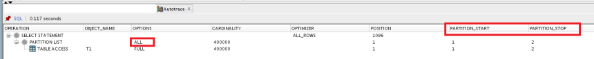
select * from t3;
This is our base test: select all data from our partitioned table:

Second scenario:
select * from t3
where c1='BCD';
Selecting data filtering on a partition key, but a value which does not exist in the table.

Third scenario:
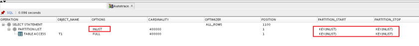
select * from t3
where c1='ABC';
Selecting data filtering on a partition key, on a valid value

Third scenario:
select * from t3
where c2 <
     (select /*+ no_unnest + result_cache*/
            (to_Date ('05-OCT-2016', 'dd-mon-yyyy')) + 1
      from dual)
;
Filtering on multiple values of our sub-partition key :

Conclusions:
I’ve been using the SQLDeveloper Autotrace to demonstrate the partition pruning.
As you can see, the selects will do partition pruning when filtering on one or multiple partitions.
But, most interesting, the database will do partition pruning when filtering directly on the sub-partition key.