Oracle Bitmap Index

Common usage of Bitmap Indexes is a data warehousing environment. This implies large amounts of data, high level of ad-hoc queries but a low level of concurrent DLM transactions.

Why to use?

  • reduced response time
  • reduced storage requirements compared to other indexing techniques
  • efficient maintenance during parallel DML and load

Bitmap indexes are typically only a fraction of the size of the indexed data in the table.

How it works?

An index provides pointers to the rows in a table that contain a given key value. A regular index stores a list of rowids for each key corresponding to the rows with that key value. In a bitmap index, a bitmap for each key value replaces a list of rowids.

Each bit in the bitmap corresponds to a possible rowid, and if the bit is set, it means that the row with the corresponding rowid contains the key value. A mapping function converts the bit position to an actual rowid, so that the bitmap index provides the same functionality as a regular index. Bitmap indexes store the bitmaps in a compressed way. If the number of distinct key values is small, bitmap indexes compress better and the space saving benefit compared to a B-tree index becomes even better.

Best use case?

From my opinion, bitmaps are most effective on queries with multiple where clauses.  As the bitmaps from bitmap indexes can be combined quickly, it is usually best to use single-column bitmap indexes. This is why the DW environment is the “home” for this type of indexing.

Frequent use cases?

The advantage of bitmap indexes is higher on columns where degree of cardinality (number of distinct values for the indexed column versus the total number of rows in the table) is small. Columns like Status, gender are optimal examples.

However, the datawarehouse environments can also benefit from bitmaps on columns with higher cardinality. This is also mostly due to the combining of bitmaps for quick filtering.

This is due to the fact that AND and OR conditions in the where clause can we resolved faster by performing Boolean operations directly on the bitmaps before converting them to rowids for data retrieval.

Using this bitmap merge methodology, Oracle can provide sub-second response time when working against multiple low-cardinality columns.

Unlike most other indexing, bitmap indexes include rows that have the null values.

Bitmap and Partitioning

You can create bitmap indexes on partitioned tables but they must be local to the partitioned table—they cannot be global indexes.

Example

create table test_tb
( row_id number
, text varchar2(100)
, status char(6));

create bitmap index test_bmpidx on test_tb(status);

On partitioned tables:

create table 
 t2
(c1 char(3) not null
, c2 date not null
, c3 number
, c4 varchar2(100))
partition by range(c2)
interval (numtodsinterval (1,'day'))
 (
 partition empty values less than (to_Date ('03-OCT-2016', 'dd-mon-yyyy'))
 )
;

create bitmap index test_bmpidx on test_tb(status);


Restrictions

You cannot create a bitmap join index on a temporary table.


Advertisement

Oracle: Partitioning and Indexes 

As I’ve been presenting in the last couple of posts on partitioning, one of the major benefits of this database option is basically the selectivity when filtering on the partition key, what we currently call partition pruning.

Now, what we’ve been experimenting with so far are simple based table. However, in the data warehousing world, things are not so simple.
One of the most common “performance fixes” that we see in DW is indexing. However, indexing is not always good, and combined with partitioning, it might prove to be a very unfortunate combination, if not done properly.

Partitioning world gives us two options in indexing:

  • Local indexing
  • Global indexing

Basically, a local index will behave similar to a partition table, being split into partitions and best performing within partition pruning cases.
The global index, on the other side, will behave like a regular index, with one particularity: when used, it will disable the partition pruning.

Basically, from my tests so far, global indexes and partition pruning don’t mix.

How and Which

The following section will provide you a simple tested guideline on how to mix these two database performance hacks to reap the highest value out of your implementation.

Unique indexes should be global – when we use unique indexes, the selectivity provided by them should be much higher than the one from partition selectivity

Non-unique indexes – local indexes – for more skewed data across partitions. This is perfect  in combination with partition pruning.

Scenario 1: Global non-unique index

Use the table T1 created as part of post Oracle: Partition by List – Example

Create index on the date column:

SQL:

create index t1_dt on t1(c2);

Now looking at regular SQL for selecting a partition and then filtering on the date column:

select * from t1
where 1=1
and c1 in ('ACD')
and c2 between trunc(sysdate) and trunc(sysdate+1);

global-non-unique-index

Create local index on the date column (drop the prior created index):

SQL:

drop index t1_dt;
create index t1_dt on t1(c2) local;

Now looking at same SQL for selecting a partition and then filtering on the date column:

select * from t1
where 1=1
and c1 in ('ACD')
and c2 between trunc(sysdate) and trunc(sysdate+1);

local-non-unique-index


Oracle: Partition by List Sub-Partition by Range– Example

The following post will walk you trough an exercise of creating a partitioned table, using the list partitioning, with range sub-partitioning (explicit definition of partitions and sub-partitions naming), populating and testing the partition pruning.

Please note I will also post the scripts at each section so you can replicate the work.

Creating our Work Table:

I’m creating a sample table T2 with 4 columns, with the following structure:

table-structure

SQL:

create table 
 t
(c1 char(3) not null
, c2 date not null
, c3 number
, c4 varchar2(100))
partition by list (c1)
subpartition by range(c2)
 (
  partition P1 values ('ABC')
 ( subpartition p1_20161003 values less than (to_date('04-oct-2016','dd-mon-yyyy'))
 , subpartition p1_20161004 values less than (to_date('05-oct-2016','dd-mon-yyyy')) , subpartition p1_20161005 values less than (to_date('06-oct-2016','dd-mon-yyyy'))
 , subpartition p1_20161006 values less than (to_date('07-oct-2016','dd-mon-yyyy'))
 , subpartition p1_20161007 values less than (to_date('08-oct-2016','dd-mon-yyyy'))
 , subpartition p1_20161008 values less than (to_date('09-oct-2016','dd-mon-yyyy'))
 , subpartition p1_20170101 values less than (to_date('01-jan-2017','dd-mon-yyyy'))
 )
 , partition P2 values ('ACD')
 ( subpartition p2_20161003 values less than (to_date('04-oct-2016','dd-mon-yyyy'))
 , subpartition p2_20161004 values less than (to_date('05-oct-2016','dd-mon-yyyy'))
 , subpartition p2_20161005 values less than (to_date('06-oct-2016','dd-mon-yyyy'))
 , subpartition p2_20161006 values less than (to_date('07-oct-2016','dd-mon-yyyy'))
 , subpartition p2_20161007 values less than (to_date('08-oct-2016','dd-mon-yyyy'))
 , subpartition p2_20161008 values less than (to_date('09-oct-2016','dd-mon-yyyy'))
 , subpartition p2_20170101 values less than (to_date('01-jan-2017','dd-mon-yyyy'))
 ) ) ;

We want to partition this table by the C1 column, and subpartition by C2 column, which is a date column: not null, splitting the data into a priorly-defined number of categories.

I’m generating a sample data set of about 100 000 rows.

table-partition-and-subpartition-after-insert

And afterwards, please note a very important step, I’m gathering my stats 🙂

insert into t3 
select 
 case 
 when mod(level,20) <11 then 'ABC'
 when mod(level,20) >10 then 'ACD'
 end as c1
 , to_date('04-oct-2016','dd-mon-yyyy')+level/24/60 
, level 
, 'test record '||level 
from dual 
connect by level <=100000; 

commit; 

execute dbms_stats.gather_table_stats(user,'T3');

Partition Pruning:

Now, let’s run a couple of test to see  how partition is actually helping our performance.

Please note that i used “Autotrace” to show the actual plan and the partition pruning for our selects.

First scenario:

select * from t3;

This is our base test: select all data from our partitioned table:

full-table-scan

Second scenario:

select * from t3
where c1='BCD';

Selecting data filtering on a partition key, but a value which does not exist in the table.

filter-by-partition-key-invalid-value

Third scenario:

select * from t3
where c1='ABC';

Selecting data filtering on a partition key, on a valid value

filter-by-partition-key-valid-value

Third scenario:

select * from t3
where c2 <
     (select /*+ no_unnest + result_cache*/
            (to_Date ('05-OCT-2016', 'dd-mon-yyyy')) + 1
      from dual)
;

Filtering on multiple values of our sub-partition key :

filter-by-subpartition-key

Conclusions:

I’ve been using the SQLDeveloper Autotrace to demonstrate the partition pruning.

As you can see, the selects will do partition pruning when filtering on one or multiple partitions.

But, most interesting, the database will do partition pruning when filtering directly on the sub-partition key.

Working with Large Data Volumes – Partitioning

As more and more the increase in information is getting visible to each database user, there comes a question on how are we to process these volumes in a Data Warehouse environment.

One of the first answers provided by Oracle on this topic is Partitioning.

What is Partitioning?

Similar to an Operating System partitioning, from a database perspective, we should envision partitioning as a logical division of data into separate units (like smaller tables). This allows the database to manage, to a certain extent, information on each partition as if it were a distinct table. Doing this, implies operating smaller sections of data, improving efficiency.

Partitioning enables tables and indexes to be subdivided into individual smaller pieces. Each piece of the database object is called a partition. A partition has its own name, and may optionally have its own storage characteristics.

From the perspective of a database administrator, a partitioned object has multiple pieces that can be managed either collectively or individually. This gives the administrator considerable flexibility in managing a partitioned object.

However, from the perspective of the application, a partitioned table is identical to a non-partitioned table; no modifications are necessary when accessing a partitioned table using SQL DML commands. Logically, it is still only one table

A query-rewrite view on an union all select of identical tables (from structure perspective)

So, to a certain extend, I would compare a partitioned table with a view on multiple tables which have the same structure (and you don’t need to bother in defining each table with the same structure, just adding a partition will give it same metadata), with a special column that sorts/tells you a critical selectivity criteria for that particular data set in the entire view, and which allows query rewrite.

Why?

Looking at a view containing multiple tables, if we query, through the view, information from only one table, Oracle knows to do a very neat trick of query rewrite, and re-writes your query into a selection from only that particular table. This allows for better performance results.

Well, partitioning does something similar, in the context of selecting from one single (or a selection of) partition(s), when filtering on the partitioning key. This is called partition pruning.

Partitioning types

In Oracle, there are a couple of major partitioning types, given a certain key/column:

  • Range Partitioning The data is distributed based on a range of values.
  • List Partitioning The data distribution is defined by a discrete list of values.
  • Hash Partitioning An internal hash algorithm is applied to the partitioning key to determine the partition.

Also, it allows sub-partitioning, which is a combination of the primary partitioning types. This is called Composite Partitioning. First, the table is partitioned by data distribution method one and then each partition is further subdivided into sub-partitions using the second data distribution method.

Additional methods of partitioning:

  • Multi-Column Range Partitioning: An option for when the partitioning key is composed of several columns and subsequent columns define a higher level of granularity than the preceding ones.
  • Interval Partitioning: Extends the capabilities of the range method by automatically defining equi-partitioned ranges for any future partitions using an interval definition as part of the table metadata.
  • Reference Partitioning: Partitions a table by leveraging an existing parent-child relationship. The primary key relationship is used to inherit the partitioning strategy of the parent table to its child table.
  • Virtual Column Based Partitioning: Allows the partitioning key to be an expression, using one or more existing columns of a table, and storing the expression as metadata only.
  • Interval Reference Partitioning: An extension to reference partitioning that allows the use of interval partitioned tables as parent tables for reference partitioning.
  • Range Partitioned Hash Cluster: Allows hash clusters to be partitioned by ranges.

How it Works?

For examples on some of the mentioned partitioning methods, please see my following posts:

See also sub-partitioning examples :

Why to use it?

Partitioning:

  • Increases performance by only working on the data that is relevant.
  • Improves availability through individual partition manageability.
  • Decreases costs by storing data in the most appropriate manner.
  • Is easy as to implement as it requires no changes to applications and queries.

References:

Please note I’ve used the official Oracle documentation for the definitions used in this post for each of the partitioning types, as well as the well known benefits. You can find the original page here.

Oracle: Partition by Range– Example

The following post will walk you trough an exercise of creating a partitioned table, using the range partitioning (with auto define of partition names), populating and testing the partition pruning.

Please note I will also post the scripts at each section so you can replicate the work.

Creating our Work Table:

I’m creating a sample table T2 with 4 columns, with the following structure:

table-t2-structure

SQL:

create table 
 t2
(c1 char(3) not null
, c2 date not null
, c3 number
, c4 varchar2(100))
partition by range(c2)
interval (numtodsinterval (1,'day'))
 (
 partition empty values less than (to_Date ('03-OCT-2016', 'dd-mon-yyyy'))
 )
;

We want to partition this table by the C2 column, which is a date column: not null, splitting the data into a non-prior-defined number of categories.

I’m generating a sample data set of about 100 000 rows.

table-t2-auto-generated-partitions

And afterwards, please note a very important step, I’m gathering my stats 🙂

insert into t2 
select 
 case 
 when mod(level,20) <11 then 'ABC'
 when mod(level,20) >10 then 'ACD'
 end as c1
 , sysdate+level/24/60
 , level
 , 'test record '||level
from dual
connect by level <=100000;


commit;

execute dbms_stats.gather_table_stats(user,'T2');

Partition Pruning:

Now, let’s run a couple of test to see  how partition is actually helping our performance.

Please note that i used “Autotrace” to show the actual plan and the partition pruning for our selects.

First scenario:

select * from t2;

This is our base test: select all data from our partitioned table:

select-all

Second scenario:

select * from t2
where c1='ABC';

Selecting data filtering on a non-partition key.

select-all-when-filter-on-non-partition-key

Third scenario:

select * from t2
where c1 =
     (select /*+ no_unnest + result_cache*/
            (to_Date ('05-OCT-2016', 'dd-mon-yyyy'))
      from dual)
;

Filtering on one of the values of the partition key, ’05-OCT-2016′:

select-1-partition-filtering-on-partition-key

Third scenario:

select * from t2
where c1 <
     (select /*+ no_unnest + result_cache*/
            (to_Date ('07-OCT-2016', 'dd-mon-yyyy'))
      from dual)
;

Filtering on multiple values of our partition key :

select-multiple-partitions-filtering-on-partition-key

Conclusions:

I’ve been using the SQLDeveloper Autotrace to demonstrate the partition pruning.

As you can see, the selects will do partition pruning when filtering on one or multiple partitions.

Also, please note the initially defined partitions are names as expected, while the rest of the data, on insert, generated automatically new partitions, named by the system.

Oracle: Partition by List – Example

The following post will walk you trough an exercise of creating a partitioned table, using the list partitioning, populating and testing the partition pruning.

Please note I will also post the scripts at the end of the post, so you can download to replicate the work.

Creating our Work Table:

I’m creating a sample table T1 with 4 columns, with the following structure:

table-t1-structure

SQL:

create table 
 t1
(c1 char(3) not null
, c2 date
, c3 number
, c4 varchar2(100))
partition by list (c1)
 (
 partition ACB values ('ABC')
 , partition ACD values ('ACD')
 )
;

We want to partition this table by the C1 column, which is more, what i call, a Category column: not null, splitting the data into a couple of finite categories. In our case we have 2 categories: ‘ABC’ and ‘ACD’:

I’m generating a sample data set of about 400 000 rows, in this particular case, evenly split between the two partitions.

And afterwards, please note a very important step, I’m gathering my stats 🙂

insert into t1 
select 
 case 
 when mod(level,20) <11 then 'ABC'
 when mod(level,20) >10 then 'ACD'
 end as c1
 , sysdate+level/24
 , level
 , 'test record '||level
from dual
connect by level <=400000;


commit;

execute dbms_stats.gather_table_stats(user,'T1');

Partition Pruning:

Now, let’s run a couple of test to see  how partition is actually helping our performance.

Please note that i used “Autotrace” to show the actual plan and the partition pruning for our selects.

First scenario:

select * from t1;

This is our base test: select all data from our partitioned table:

select-all

Second scenario:

select * from t1
where c1='ABC';

or

select * from t1
where c1='ACD';

Filtering on one of the values of the partition key, ‘ABC’:

select-abc-only

Third scenario:

select * from t1
where c1 in ('ABC', 'ACD');

Filtering on both values of our partition key (‘ABC’ and ‘ACD’):

select-both

Conclusions:

I’ve been using the SQLDeveloper Autotrace to demonstrate the partition pruning.

As you can see, the selects will do partition pruning when filtering on one or multiple partitions.

Scripts:

test-scripts

Please note scripts are uploaded as PDFs but you can still copy the code in.

Slowly Changing Dimensions – explained

Overview

In discussing Slowly Changing Dimension, the first thing you must consider is first of all, your attributes type. Base on this, you will have various SCD types or combination of types.
Dimension Attribute Types:

  1. Type 0: dimension attribute that never changes.
  2. Type 1: dimension attribute that is overwritten with new values/changes
  3. Type 2: dimension attribute on which we track changes of a value ( for same logical tuple in the table, you will have multiple records representing the changes occurring on that column).

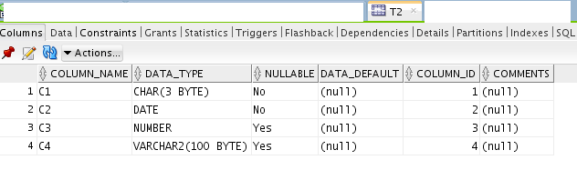
To discuss the various types of columns, let’s take a more generic table example.
We have table DEMO_SCD created for this purpose, with following structure:Overview 1And have inserted a couple of test records/tuples for this:Overview 2In the following definitions, I will define a logical tuple as information identified in a record or records by the natural key.

Dimension attributes types

Type 0 – never changing

These will represent the columns that stay in their original state all the time. This does not imply though that new values of this column cannot be introduced into the dimension. It implies only that for a logical tuple, the information will never change in time, independently of the other columns information for the given table.

One example for this type is the audit creation columns (created by, created date), which will not be changes when the information in the main table changes.
Another example is the natural key of the table (in our test table the ROW_CODE).

The overall constraint on this type is the fact that the information once inserted, it will not change in time.

Type 1 – Volatile Value

These will represent the columns that will change in time, losing the original state. Information can be added, deleted or modified at will. This implies that for a logical tuple, the information will always contain the current/most recent data.

An example of this type of columns represents the audit update columns (last update date, last updated by), whose scope is to capture the last person manipulating a tuple.

Type 2 – Versioning Values

These are columns on which the evolution in time of the value is of interest to the analyst. This implies that values for this column can be inserted, but never updated or deleted. However, this also implies that additional columns are required to implement this, in order to keep track of versioning history, and be able to identify the current data.
I am going to cover only 2 of the implementation options possible:

  • Versioning
  • Time based / Active time range /effective dates

Versioning

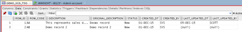
Versioning containing tables will look like the following example:Versioning 1
Please note the tuple of AA, where the change in status generated a second record with an increased version number.
Versioning 2
Please note here the VERSION column, which keeps track of the changing of data.
On joining with a versioned SCD, a fact table would have to join by

  • Surrogate key – ROW_ID – this way the identification of correct version is done on populating the fact, and not at reporting time)
  • Natural key and version number
  • Natural key and maximum version (if we report only on current data)
  • Natural key and 0 version (if we report on original data)

Effective Dates

Implementation using effective dates would imply the existence of 1 or 2 date columns which would identify the period the record is active for.

Since the implementation containing one date column would make the identification of a specific information/version of a tuple at a given point in time more difficult, I would always suggest the implementation containing two date columns.
Effective Date 1
Same change on tuple AA is now represented in this example
Effective Date 2
Please note here the START_DATE and END_DATE columns, which keep track of the changing of data.

On joining with a time based SCD, a fact table would have to join by

  • Surrogate key – ROW_ID – this way the identification of correct version is done on populating the fact, and not at reporting time)
  • Natural key and join on start_Date, end_date columns
  • Natural key and current version(identified by end_date null) (if we report only on current data)

Please note that both type 2 columns implementation involve:

  • Updating current record for working tuple
  • Inserting new record with different surrogate key for working tuple

Dimension types

Now, based on the analysis of the column types, we can identify multiple versions of SCD

  • Type 0 – only Type 0 columns;
  • Type 1 – contains type 0 and 1 columns;
  • Type 2 – contains type 2 columns;
  • Type 3 – contains type 2 columns;
  • Type 4 – contains type 2 columns;
  • Type 6 – contains type 2 columns;

Type 0 – Static Tables

This type of table is, from what I see, rarely found in a Data warehouse, but the most frequent example would be a log table. This type of dimension would have data that only gents inserted, and never gets modified.

Type 1 – Current Data Tables

These are the tables where we’re only recording the current version of events. Every single update will modify the exiting tuple in the table, and no historical reporting is possible on this scenario.

Type 2

This type tracks history by creating multiple entries for a given tuple. Unlimited history is preserved for each.
Implementation examples for this are the ones presented for the Type 2 columns.

Type 3

This method will only keep a limited history for each tuple.

The implementation implies additional columns that will keep the last value of a given attribute that we are tracking, or the original state of that column.
This is however very limited, as multiple changes on the same tuple will not be tracked.

Example for this type:
DM type 3 - 1
Please note the ORIGINAL_DESCRIPTION column capturing the original information for the description of the tuple at the time this was created.
DM type 3 - 2
Please note in this example the PRIOR_STATUS. In this implementation, we will only track the last change; the original value will no longer be available for reporting.

Type 4

This is a slightly different scenario, involving 2 tables to keep the tuple information:

  • Current table – only current information
  • History table – part of or all historical information

Both tables will have to be used in reporting, by joining with the fact with each table’s surrogate key.

Example of current table implementation:
DM type 4 - 1
and associated history table:
DM type 4 - 2

Note the AA tuple within the 2 tables.

Type 6

The Type 6 method combines the approaches of types 1, 2 and 3 (1 + 2 + 3 = 6). Ralph Kimball calls this method “Unpredictable Changes with Single-Version Overlay” in The Data Warehouse Toolkit.
DM type 6
Please note data modifications for tuple identified by ROW_CODE = ‘AA’
You will notice that for current record (current flag is ‘Y’), the current status and historical status as always the same.

Note also that the tuple can pass multiple times through the same status.


General classification source: Wikipedia